“How do you create a linear programming model in Excel?”
- Create a formula for your objective
- Determine your decision variables
- Set your constraints
- Enter all of the above into Solver
- Run Solver in your spreadsheet
Linear programming, integer programming, quadratic programming, and other similar concepts are probably more mathematical in nature than business-centric. However just because they are complicated doesn’t mean that they can’t serve businesses needs.
Let me begin this explanation of linear programming with a qualifier. I’m not a mathematician, I’m a management accounting expert. So keep that in mind as you read this – I’m explaining things as best I can. But I admittedly don’t have a complete understanding of these concepts.
At its foundation, linear programming is a means of finding an optimum solution. As business people, we try to make the best decisions we can with the information we have. However, no matter how adept we might be at our craft we don’t have CPUs implanted in our brains. And because of this, we’re probably not always making optimum decisions.
Though the math behind linear programming is somewhat complicated. The concepts behind it are fairly simplistic.
Ultimately, we’re simply looking for the undisputed best solution for a given problem. Even if we don’t completely understand how it’s calculated. None of us are in any position to turn down the absolute best solution to our problems.
So let’s get a little bit further into the guts of linear programming.
Looking for more spreadsheet templates?
Linear programming worksheet download
Complete the form below and click Submit.
Upon email confirmation, the workbook will open in a new tab.
How do you create a linear programming model in Excel?
You’ll notice that the linear programming worksheet has three distinct sections. Objective, Decision variables, and Constraints.
Due to linear programming’s unique mathematical nature, performing linear programming functions in spreadsheets requires special software.
In Excel that special software is known as Solver. Here’s how to load the Solver add-in into Excel.
For Google Sheets, you will need a special add-on also. This is one of the better-reviewed add-ons, called OpenSolver.
For OpenOffice Calc, the add-in is also called Solver. Solver comes pre-installed with OpenOffice Calc. Just go to Tools > Solver.
*Since this example might be a bit too complicated for the Google Sheets and OpenOffice Solvers. If you want to play around with this workbook, you’ll probably need to use the Excel Solver and try different “Solving Methods.”
Again, linear programming has a wide array of practical applications. This workbook merely serves as an example, not a template per se. You could, in theory, apply it to your business. But, it’s unlikely that it would be an exact fit for you. If you want to implement linear programming in your business, you’ll probably have to build something yourself or hire a 3rd party to help you.
Objective
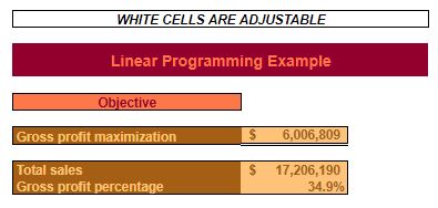
The Objective is exactly what it sounds like. This is where you specify what it is that you want to maximize, minimize, or reach an exact value for.
Your Objective cell will consist of a formula. Because, of course, your Objective will be affected by several different variables. It’s up to you to build the formula for your Objective. It’s up to the linear programming add-in to optimize your Objective.
Gross profit maximization
The example workbook only scratches the surface of what linear programming is capable of. The number of problems that linear programming can solve (assuming that they aren’t illogical) is nearly limitless.
How to allocate costs more accurately.
This example is going to keep things simple. So, I’m going to use a dummy company that is tied to my previous workbooks. This company’s goal is to maximize its gross profit within the specified constraints.
Gross profit is the result of (Price Per Unit – Matl Cost Per Unit – DL Cost Per Unit – OH Cost Per Unit) × the quantity sold of each item.
Also included in this section, is Total sales and Gross profit percentage. These are included only to provide context and perspective for Gross profit maximization. They will have no bearing on the Optimum Quantity.
Total sales
Total sales are simply the sum of Price Per Unit × Optimum Quantity for every item.
Gross profit percentage
Gross profit maximization ÷ Total sales.
Decision variables
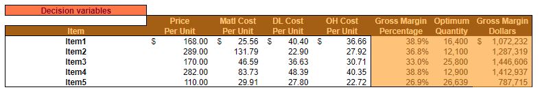
The Decision variables are exactly what they sound like. They represent the decisions that your company has to make. I told you that, at its core, this was not a terribly complicated thing. The computer handles the intensive math – you just need to enter the inputs.
The Decision variables are up to you. In this example, you decide how much you want to charge for each item (Price Per Unit).
You also decide (kind of) what your cost will be for material, direct labor, and overhead. These amounts will play the biggest part in deciding what the optimum quantities are. And, therefore, what your maximum gross profit is.
Item, Price Per Unit, Matl, DL, and OH Cost Per Unit
These fields are pretty straightforward.
You probably know, with a good degree of certainty, what’s your Price Per Unit is.
You can probably estimate (if you don’t already know) what your Material Cost Per Unit is.
Direct labor is where it starts to get tricky. If you have solid cost accounting, then you can probably get an accurate idea of what your DL Cost Per Unit is.
Overhead is where we really start getting into subjective territory. First, what do you include in overhead? Second, how do you allocate overhead to each unit? Again, solid cost accounting will help put your mind at ease here.
Things to consider when allocating overhead
Depending on the nature of your business, overhead could make up a significant portion of your costs – thereby greatly affecting the Optimum Quantity and subsequently your maximum gross profit.
If your cost accounting sucks then you’re going to have to rely on a best guess. I would suggest you focus more on allocating overhead across items in a proportion that you’re comfortable with rather than dwelling on the cost per unit for overhead.
What do I mean by that? If, intuitively, you know that Item1 is responsible for twice as much overhead cost as Item2, then make sure that your OH Cost Per Unit is twice as much for Item1. Whether that means a cost of $100, or $1 doesn’t matter as much. What matters is that it’s 2x as much relative to Item2.
The reason being that, at the core of this analysis, you’re really trying to decide how much of each item to sell – given your constraints. All items are in competition with each other. So while an accurate OH Cost Per Unit is desirable; it’s really most important for you to understand which items are burdened with the most overhead.
Should you be using the FIFO or weighted-average method with process costing?
Gross Margin Percentage, Optimum Quantity, & Gross Margin Dollars
Gross Margin Percentage
(Price Per Unit – Matl Cost Per Unit – DL Cost Per Unit – OH Cost Per Unit) ÷ Price Per Unit
In other words, gross margin for each item ÷ Price Per Unit
Optimum Quantity
There is no formula in the Optimum Quantity fields. If you’re familiar with Spreadsheets for Business’s Excel templates, then you might be wondering why Optimum Quantity isn’t in white?
It’s because the Optimum Quantity is not for you to input. Again, this is a linear programming (ie an optimization) workbook. With all due respect to you, brilliant user, it would probably take you a long time to find the Optimum Quantities via trial and error.
So, these cells are shaded because these are the cells that the linear programming add-in will make changes to determine what Optimum Quantities will result in Gross profit maximization.
Gross margin dollars
Price Per Unit × Gross Margin Percentage × Optimum Quantity.
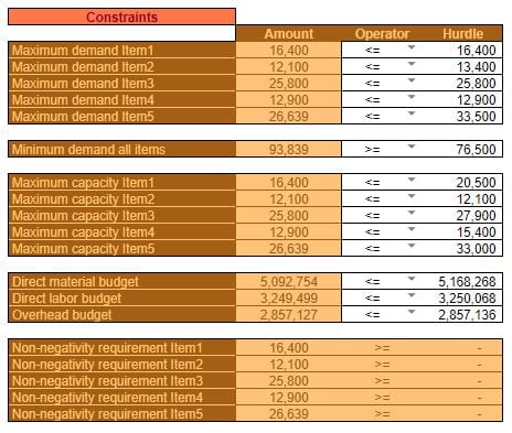
Constraints
The constraints are (also) exactly what they sound like.
Obviously, if we’re trying to maximize something – the ideal situation is to simply do as much as we can. Your business could maximize net profit by simply selling an infinite amount of something with a 100% gross margin. Easy right?
Of course, it’s not that easy. Constraints are a reality of business and life in general. Demand is a constraint. Time is a constraint. Manpower is a constraint. I could go on and on. There is no shortage of constraints in this world.
Therefore, when we seek an Objective we must work within the confines of those Constraints. Not to say that those Constraints can’t change at some point in the future. But at this point in time, they are what they are and we’re going to have to work around them.
Again the Constraints in this linear programming example are going to revolve around Gross profit maximization. So let’s look at those constraints in a little more detail.
Maximum demand
Maximum demand is a constraint of course because we can’t sell any more than customers are willing to buy (unfortunately).
If we refer back to the operating budget we’ll remind ourselves of what we had forecasted in terms of demand for each item. Obviously, the Maximum demand needs to be above those quantities. Otherwise, we need to go back and tweak our operating budget – because we’re not going to sell more than the Maximum demand.
Once you’ve come to terms with an acceptable Maximum demand for each item, enter that quantity under the Hurdle heading. When we run the linear programming add-in, the Amount that we hope to sell for each item should not exceed this Hurdle amount.
The Operator field is pretty simple and straightforward. You’ll see that it’s a drop-down menu that allows you to choose ≤, =, or ≥. In this example, since we’re dealing with maximum demand then we want the Operator to be “≤” for all Maximum demand Constraints.
Quick and easy tool for measuring customer profitability.
Finally, the Amount for each item is equal to the Optimum Quantity from the Decision variables section.
Minimum demand
Minimum demand was included as a Constraint just to demonstrate how the Decision variables can have a lower bound along with an upper bound.
Of course, for most businesses, the Minimum demand is zero. But, that gets addressed later in the non-negativity requirements. So for the sake of an example, a minimum total quantity Constraint was added because there might be a situation where a business had a shipping contract or something of the like. Hell, maybe the Minimum demand is the total amount of units forecasted to be sold in the operating budget?
A quantity for Minimum demand is entered as the Hurdle. The Operator, in this case, is, of course, “≥.” And, the Amount is equal to the sum of all of the Optimum Quantities from the Decision variables section.
Maximum capacity
Maximum capacity isn’t a conceptual constraint. It is very real. You, quite simply, can not produce more than your resources will allow. That is – unless you retain more resources.
Capacity constraints might come in the form of material, labor, machinery, or something else.
In this example, it was assumed that my capacity limitations weren’t too constricting. An appropriate Hurdle is entered for each capacity restriction, for each item.
Make a note that in some cases my Maximum capacity is above my Maximum demand. This means that I have excess (and useless) capacity. In other instances, Maximum capacity is less than Maximum demand. This means that I am leaving potential sales on the table because I don’t have the resources to keep up with demand.
In either case, Maximum demand or Maximum capacity will set an upper limit on the number of a particular item that I can sell.
Budgetary constraints
Budgetary constraints aren’t as firm as capacity constraints. But, the whole point of creating a budget is to put self-imposed constraints on your spending. So, including them in a linear programming exercise, such as this, make sense.
Again if you’re following along and have reviewed the operating budget, you’ll notice that the Hurdle amounts for the Direct material, Direct labor, and Overhead budget come directly from that workbook.
Obviously, you can overspend on these budgets. But if you went to all the effort of creating an operating budget then it makes sense to try to optimize gross profit within those constraints.
The Operator, of course, is “≤.” This is because we want to keep the spending amount below what we budgeted.
How do we determine the Amount for direct materials, direct labor, and overhead? Because of the information entered above in the Matl Cost Per Unit, DL Cost Per Unit, and OH Cost Per Unit fields.
Those amounts are taken times the Optimum Quantity to ascertain how much is spent in each category.
Non-negativity requirements
The final constraint is one that doesn’t require any thinking on your part.
In most circumstances, a negative amount of any Decision variable is unrealistic. You can’t produce or sell negative quantities.
Granted, since linear programming is so versatile, there could potentially be situations where it would make sense to have negative Decision variables. But, obviously, for what we are trying to accomplish in this example, allowing negative Decision variables doesn’t make sense.
The Amount pulls from the Optimum Quantities above. Of course, the Operator is “≥” to the Hurdle amount of 0, for all items.
Make sure you’re dealing with integers
One final Constraint to keep in mind is to make sure that your Decision variables remain integers. Just like with the Non-negativity requirement, you can’t (usually) make or sell a fractional quantity of a product. For example, sales quantities can’t be 1.234, 2.5, or 4.899938. They have to be 1, 3, and 5, respectively.
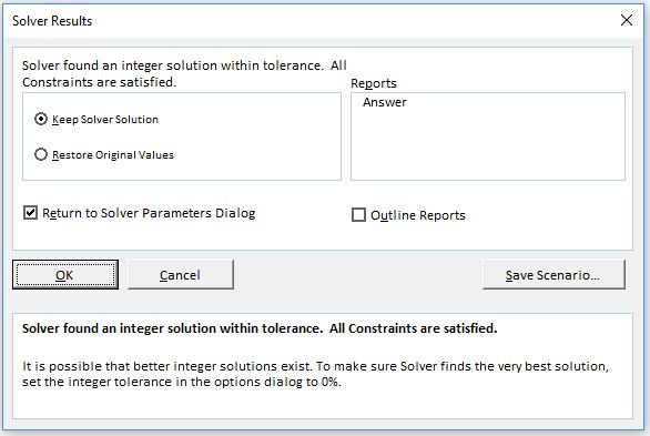
When you run the Solver add-in it will use fractional amounts unless you tell it otherwise. It’s only concerned with trying to find the optimal solution within the Constraints you outlined. Make sure you specify as a Constraint, that each Decision variable must be an integer.
Quantity and Gross Margin chart
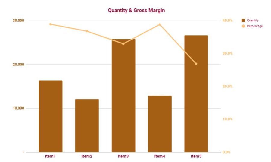
The Quantity & Gross Margin chart is a simple representation of the results of running the linear programming equations.
The Optimum Quantities are represented by the bars and charted on the left axis. The Gross Margin Percentage for each item is represented by the line and is charted on the right Axis.
How to run Solver in Excel, Google Sheets, and OpenOffice
Linear programming add-ins are available for Excel, Google Sheets, and OpenOffice Calc. For each piece of software, the add-in is known (typically) by the name “Solver.”
Full disclosure I’ve only ever used Solver in Excel for any length of time. I haven’t used the Solver add-on for Google Sheets much. Nor have I used Solver in OpenOffice more than once. My impression is that they all look, more or less, the same and operate in a very similar manner.
Google Sheets has a couple of different options for linear programming add-ons. The most popular looks to be one that’s called OpenSolver.
No matter which piece of software, or which add-in you decide to use, the fundamentals are the same for all of them. Each will require similar inputs in order for the Solver to run.
That being said, I would suggest using Excel for this type of analysis.
The SFB – Linear Programming workbook can be downloaded into Excel from Google Sheets by selecting File > Download as > Microsoft Excel (.xlsx) from the main menu.
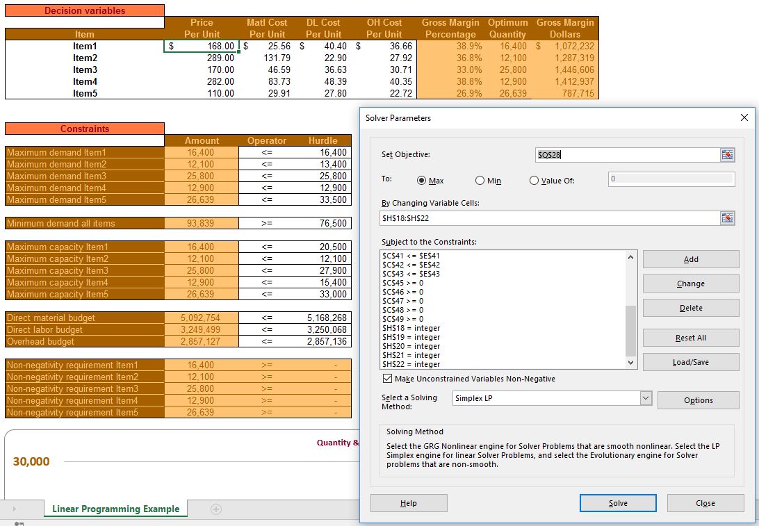
Set Objective
The first bit of business to settle on is your Objective. This will be one cell within your workbook and it is in the focus of the entire exercise of linear programming.
In the case of the example the Objective, of course, is Gross profit maximization.
Max, Min, or Value Of
The next step is to choose whether you want to maximize, minimize, or meet a specific value in the Objective cell.
Obviously, it depends on the nature of your analysis as to which choice you would make. In my example, since I am trying to maximize gross profit, of course, I chose “maximize.”
Variable Cells
Variable cells are what can be changed in order to affect your Objective.
The variable cells can’t be a formula. They need to be numeric inputs. These are the cells that affect all the other formulas in your worksheet. So, they’re not affected by anything else that might be changed.
Subject to the Constraints
Finally, with the Objective and Decision variables set, it’s time to enter the Constraints. This can be the most tedious part of setting up a linear programming operation. But, of course, it’s necessary if you want to get quality results.
For each Constraint, you’ll reference a cell and then an Operator. After that, you’ll either enter a specific amount manually, or you’ll reference a Hurdle cell.
After you attended all the Constraints, you’re ready to run Solver.
Solving Method & Options
Remember how I mentioned at the beginning of this page that I am not a mathematician?
For Solver in Excel, there are a couple of different solving methods you can employ. I don’t think that Google Sheets or OpenOffice Calc have as much versatility.
Excel offers the following solving methods: Simplex LP, GRG nonlinear, and Evolutionary. I really don’t know what the distinction is between all three. My typical course of action is to start with Simplex LP and if I get an error, then I move to GRG nonlinear. If GRG nonlinear gives me trouble then I try Evolutionary. Evolutionary seems to be able to handle about anything I throw at it – assuming that there are no logical inconsistencies.
Maybe you’re disappointed that I don’t know every detail behind each solving method? That’s fine. Frankly, I would like to know all that. But I don’t have the time, nor, possibly, the capacity to understand it.
When you finally get everything set up running you’re almost certainly going to get a better result out of Solver than you would have ever been able to come up with on your own. So whether you or I understand exactly how it works or not, all that matters is that it does.